Spatio-Temporal Parallelism

Intended audience and purpose

The ParaView Spatio-Temporal Parallel Processing Tools are designed to dramatically reduce the running time of parallel data analysis jobs under certain conditions. These conditions include:

1. The data is composed of a large amount of time steps.
2. The data analysis operations are to be applied to each time step, and time steps are independent of each other (i.e. no data exchange between time steps is required). Examples Include generating an image of each time step and creating a contour of each time step.
3. Optionally, for spatial parallelism the data for a single time step does not fit in a single core’s available memory while utilizing all cores on the processor or node.

Introduction and problem definition

In the age of “big data”, dealing with the massive amount of data can be an enormous challenge. For our definition of big data with respect to scientific computing, we are going by the working definition of data that requires an inordinate amount of time to analyze to obtain salient information on an appropriate computing platform. Often when the analysis is separate from the computation (i.e. the simulation code producing the data), disk IO can be a significant factor. According to the DOE Exascale Initiative Roadmap, Architecture and Technology Workshop in San Diego in December 2009, for supercomputers there is expected to be a 500 fold increase in the FLOP/s between 2010 and 2018 but only a 100 fold increase in the IO bandwidth in that same time. Because of this we need to concentrate on ways to efficiently post-process simulation data generated on these leading edge supercomputers.

Approach and solutions

To this end we have approached this problem by reducing the amount of global operations that need to be done to process the data. We begin with the assumption that the simulation is time dependent and will be outputting data for multiple time steps. When processing this data, similar operations will need to be done for each time step but we look to group the amount of processes that work on a time step together to a reasonable size instead of using all of the available processes. We call the set of processes working together on a time step as the time compartment. By having multiple time compartments we can ensure that there is an appropriate amount of work being done by each process. Additionally, the communication between processes is generally done within the time compartment and not over the entire global set of processes. In fact, for certain situations such as creating an image for each time step there will be no global inter-process communication. An example of this is shown in the figure below for 3 time steps and 3 time compartments of size 4. Note that for more time steps each time compartment would process multiple time steps for this example.

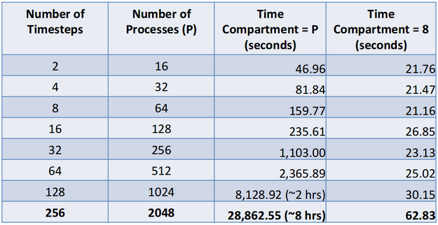
Note that the main advantage of this approach is that it escapes the typical limits of strong scaling for large amounts of processes where the computation per process gets overwhelmed by the communication per process. Similar results are obtained for weak scaling when the number of time steps analyzed is increased with process count while maintaining the same amount of work per time step. This is shown in the table below for results from the Parallel Ocean Program code (POP). Note that 1.4 GB of data is read in per time step and we compared using pure spatial parallelism (the time compartment size equal to the number of processes) and spatio-temporal parallelism with a time compartment size of 8.

This was done on Los Alamos National Laboratory's Mustang supercomputer using 8 cores per node. A time compartment size of 8 is a reasonable value for this machine as long as the data fits on a single node. The reason for this is that it limits the inter-process communication to intra-node communication. While many analyses will be time step independent (i.e. time step A and time step B don’t need to share any information), we will also have cases where there is a global reduction operation. We have tested this for some temporal statistics (average, minimum, maximum and standard deviation) but a customized solution would need to be done for each global reduction operation.

Accessing ParaView’s spatio-temporal tools

ParaView’s spatio-temporal tools are available for download from http://www.paraview.org/paraview/resources/software.php under the nightly version of ParaView. Once this is done the following steps can be followed to create a Python script with spatio-temporal parallelism. After this is done the following section discusses how to properly run the Python script. Create spatio-temporal pipeline scripts in the ParaView GUI The goal of using spatio-temporal parallelism is to reduce the time for analyzing the simulation results. Thus, a key component in the workflow is being able to create and run the scripts quickly and easily. In order to do this, we’ve developed a ParaView plugin that can generate these spatio-temporal pipeline scripts. In this section we’ll walk through the steps to create a script.

The easiest way to create a new spatio-temporal pipeline script is to use ParaView’s GUI plugin. The directions are as follows:

1. Start up the ParaView GUI.
2. In the GUI, go to the Tools menu and select Manage Plugins. In the pop-up dialogue window, select TemporalParallelismPlugin and click on Load Selected. At this point it should list the plugin as loaded. To exit this dialog, click on Close.
3. Now, go through and create a pipeline to process the data as desired. The key point here is that any data files or images that we want to have output from our script needs to be included. For data files we don’t need to store a local version, we just need to specify how to save the data when we run the script on the desired machine with the desired input files. We do this by creating a proxy to the writer that we want to use and specifying a file name to write to. Note that as we expect to write one file per time step we add in a wildcard “%t” which gets replaced with the time step index when creating the file. The steps to do this in the GUI are:
   1. Go to the STP Writers menu and select an appropriate writer. Writers that cannot be used with the data set will be grayed out and not accessible.
   2. Make sure that the writer proxy is highlighted. This is shown in the figure below where ParallelUnstructuredGridWriter is selected in the Pipeline Browser.
      
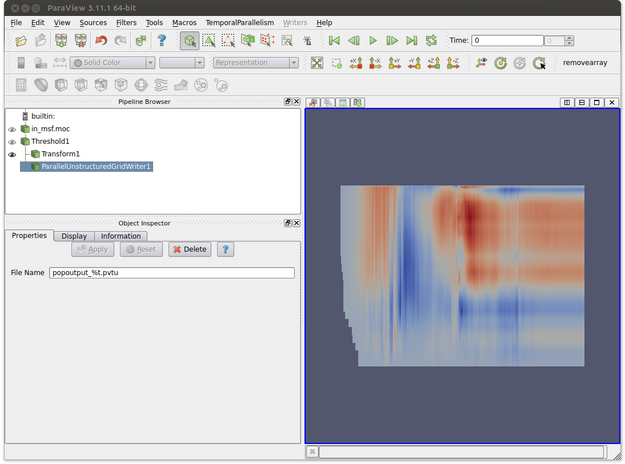
   3. In the Object Inspector, enter the name of the file. Note that %t will be replaced by the corresponding time step for each output file. In the figure below the output file name is popoutput_%t.pvtu. Note that the transform filter is used to obtain a better visual representation of the data but we would prefer to save the data in its original unscaled form.
4. At this point our script will read in a set of files, threshold out bad values (i.e. POP values that are set indicating that there is land) and write a file that contains that information. We may also want to output images based on our available view windows. This is set when we output the script. The steps to generate the script are:
   1. Click on the TemporalParallelism menu item and select Export State.
   2. This pops up a wizard to guide the user through exporting the spatio-temporal script. For the first window, click Next.
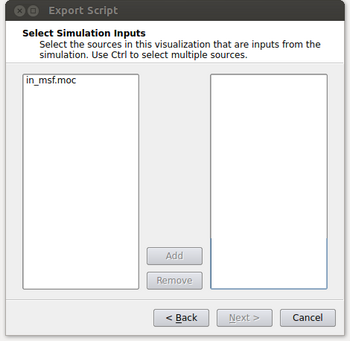
   3. At this point the window will look like the figure below. It’s possible that the user could have read in multiple files and this menu gives them the option of selecting which files they want to process in their spatio-temporal pipeline. Typically this will be a single input (in_msf.moc in this example) and the user can either double click on it or select it and click on the Add button. After this is done, click on the Next button.
      
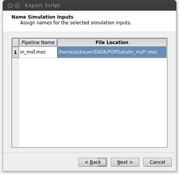
   4. At this point, we need to specify where the input is coming from on the machine we’ll be running the script on and what that input corresponds to with our local pipeline. For our example, we want the in_msf.moc source in our pipeline to read in files located at “/home/acbauer/DATA/POPData/in_msf*.moc”. The wildcard is included as we have multiple files to be read (e.g. in_msf0.moc, in_msf1.moc,...) for the machine we’ll be running on. After this is done, click on the Next button.
      
   5. At the next window, we specify the time compartment size to be used in our run. Setting a time compartment size of 1 results in each process working independently on separate time steps. A time compartment size of 1 will work well when the amount of data per time step is small. For typical supercomputers though, the amount of memory per core is relatively small such that we will also need to spatially decompose the data in order to efficiently use each core while also not running out of memory on the node. In this case the time compartment size should be the number of cores on a node or some multiple of that value as the data size per time step increases. This is shown in the figure below
      
   6. If an image is desired for the output, it needs to be specified at this point. By enabling the “Output rendering components i.e. views” option, it will allow the user to set parameters to output each view in the script as an image. The parameters are image type, the name of the file where again %t will be replaced with the corresponding time step and a magnification factor. In our example we only have a single view but if there were more the user could toggle through the views by clicking on the Previous View and Next View buttons.
      
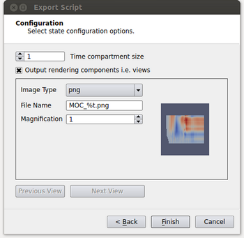
   7. After this has been done, click on the Finish button which will open a dialogue to specify the name and location to save the spatio-temoral pipeline Python script.

Run the spatio-temporal pipeline script

Now that the script has been created, the user will need to transfer the script to the machine it is intended to be run on. If the path to the input and output files aren’t known a priori and set in step 4.4 above, they may need to be changed to match where it is found on the supercomputer. As there are many different ways to run a program built with MPI (e.g. mpirun, mpiexec, aprun, etc.), the user will have to look at the machine documentation to figure that out. We assume here that mpirun is being used in which case “mpirun -np <numprocs> <install path>/bin/pvbatch --symmetric <name and location of script>” is used to run the script.

More information

We have submitted a paper to the 2013 LDAV conference. This paper develops a performance model on spatio-temporal parallelism and demonstrates its effectiveness at reducing run-time for analysis and visualization.

Acknowledgements

This work was done as part of the UV-CDAT project (http://uv-cdat.llnl.gov/) and was developed in collaboration with John Patchett and Boonthanome Nouanesengsy of Los Alamos National Laboratory.