Statistical analysis
ParaView Statistics Filters
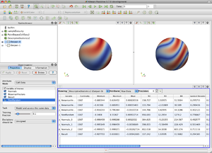
Since version 3.6.2, ParaView comes with a set of statistics filters. These filters provide a way to use vtkStatisticsAlgorithm subclasses from within ParaView.
Once ParaView is started, you should see a submenu in the Filters menu bar named Statistics that contains
- Contingency Statistics
- Descriptive Statistics
- K-Means
- Multicorrelative Statistics
- Principal Component Analysis
Using the filters
In the simplest use case, just select a dataset in ParaView's pipeline browser, create a statistics filter from the Filter→Statistics menu, hit return to accept the default empty second filter input, select the arrays you are interested in, and click Apply.
The default task for all of the filters (labeled "Model and assess the same data") is to use a small, random portion of your dataset to create a statistical model and then use that model to evaluate all of the data. There are 4 different tasks that filters can perform:
- "Statistics of all the data," which creates an output table (or tables) summarizing the entire input dataset;
- "Model a subset of the data," which creates an output table (or tables) summarizing a randomly-chosen subset of the input dataset;
- "Assess the data with a model," which adds attributes to the first input dataset using a model provided on the second input port; and
- "Model and assess the same data," which is really just the 2 operations above applied to the same input dataset. The model is first trained using a fraction of the input data and then the entire dataset is assessed using that model.
When the task includes creating a model (i.e., tasks 2, and 4), you may adjust the fraction of the input dataset used for training. You should avoid using a large fraction of the input data for training as you will then not be able to detect overfitting. The Training fraction setting will be ignored for tasks 1 and 3.
The first output of statistics filters is always the model table(s). The model may be newly-created (tasks 1, 2, or 4) or a copy of the input model (task 3). The second output will either be empty (tasks 1 and 2) or a copy of the input dataset with additional attribute arrays (tasks 3 and 4).
Caveats
Warning: When computing statistics on point arrays and running pvserver with data distributed across more than a single process, the statistics will be skewed because points stored on both processes (due to cells that neighbor each other on different processes) will be counted once for each process they appear in.
One way to resolve this issue is to force a redistribution of the data, which is not simple. Another approach is to keep a reverse lookup table of data points so that those already visited can be marked as such and not factored in a second time; this might be inefficient.
Filter-specific options
Descriptive Statistics
This filter computes the mininmum, maximum, mean, M2, M3, and M4 aggregates, standard deviation, skewness, and kurtosis for each selected array. Various estimators are available for those 3 last statistics.
The assessment of data is performed by providing the 1-D Mahalanobis distance from a given reference value with respect to a given deviation; these 2 quantities can be, but do not have to be, a mean and standard deviation, for instance when the implicit assumption of a 1-dimensional Gaussian distribution is made. In this context The Signed Deviations option allows for the control of whether the reported number of deviations will always be positive or whether the sign encodes if the input point was above or below the mean.
Contingency Statistics
This filter computes contingency tables between pairs of attributes. These contingency tables are empirical joint probability distributions; given a pair of attribute values, the observed frequency per observation is retured. Thus the result of analysis is a tabular bivariate probability distribution. This table serves as a Bayesian-style prior model when assessing a set of observations. Data is assessed by computing
- the probability of observing both variables simultaneously;
- the probability of each variable conditioned on the other (the two values need not be identical); and
- the pointwise mutual information (PMI).
Finally, the summary statistics include the information entropy of the observations.
K-Means
This filter iteratively computes the center of k clusters in a space whose coordinates are specified by the arrays you select. The clusters are chosen as local minima of the sum of square Euclidean distances from each point to its nearest cluster center. The model is then a set of cluster centers. Data is assessed by assigning a cluster center and distance to the cluster to each point in the input data set.
The K option lets you specify the number of clusters. The Max Iterations option lets you specify the maximum number of iterations before the search for cluster centers terminates. The Tolerance option lets you specify the relative tolerance on cluster center coordinate changes between iterations before the search for cluster centers terminates.
Multicorrelative Statistics
This filter computes the covariance matrix for all the arrays you select plus the mean of each array. The model is thus a multivariate Gaussian distribution with the mean vector and variances provided. Data is assessed using this model by computing the Mahalanobis distance for each input point. This distance will always be positive.
The learned model output format is rather dense and can be confusing, so it is discussed here. The first filter output is a multiblock dataset consisting of 2 tables.
- Raw covariance data.
- Covariance matrix and its Cholesky decomposition.
Raw covariances
The first table has 3 meaningful columns: 2 titled "Column1" and "Column2" whose entries generally refer to the N arrays you selected when preparing the filter and 1 column titled "Entries" that contains numeric values. The first row will always contain the number of observations in the statistical analysis. The next N rows contain the mean for each of the N arrays you selected. The remaining rows contain covariances of pairs of arrays.
Correlations
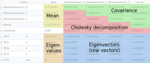
The second table contains information derived from the raw covariance data of the first table. The first N rows of the first column contain the name of one array you selected for analysis. These rows are followed by a single entry labeled "Cholesky" for a total of N+1 rows. The second column, Mean contains the mean of each variable in the first N entries and the number of observations processed in the final (N+1) row.
The remaining columns (there are N, one for each array) contain 2 matrices in triangular format. The upper right triangle contains the covariance matrix (which is symmetric, so its lower triangle may be inferred). The lower left triangle contains the Cholesky decomposition of the covariance matrix (which is triangular, so its upper triangle is zero). Because the diagonal must be stored for both matrices, an additional row is required — hence the N+1 rows and the final entry of the column named "Column".
Principal Component Analysis
This filter performs additional analysis above and beyond the multicorrelative filter. It computes the eigenvalues and eigenvectors of the covariance matrix from the multicorrelative filter. Data is then assessed by projecting the original tuples into a possibly lower-dimensional space. For more information see the Wikipedia entry on principal component analysis (PCA).
The Normalization Scheme option allows you to choose between no normalization — in which case each variable of interest is assumed to be interchangeable (i.e., of the same dimension and units) — or diagonal covariance normalization — in which case each (i,j)-entry of the covariance matrix is normalized by sqrt(cov(i,i) cov(j,j)) before the eigenvector decomposition is performed. This is useful when variables of interest are not comparable but their variances are expected to be useful indications of their full range, and their full ranges are expected to be useful normalization factors.
As PCA is frequently used for projecting tuples into a lower-dimensional space that preserves as much information as possible, several settings are available to control the assessment output. The Basis Scheme allows you to control how projection to a lower dimension is performed. Either no projection is performed (i.e., the output assessment has the same dimension as the number of variables of interest), or projection is performed using the first N entries of each eigenvector, or projection is performed using the first several entries of each eigenvector such that the "information energy" of the projection will be above some specified amount E.
The Basis Size setting specifies N, the dimension of the projected space when the Basis Scheme is set to "Fixed-size basis". The Basis Energy setting specifies E, the minimum "information energy" when the Basis Scheme is set to "Fixed-energy basis".
Since the PCA filter uses the multicorrelative filter's analysis, it shares the same raw covariance table specified above. The second table in the multiblock dataset comprising the model output is an expanded version of the multicorrelative version.
PCA Derived Data Output
As above, the second model table contains the mean values, the upper-triangular portion of the symmetric covariance matrix, and the non-zero lower-triangular portion of the Cholesky decomposition of the covariance matrix. Below these entries are the eigenvalues of the covariance matrix (in the column labeled "Mean") and the eigenvectors (as row vectors) in an additional NxN matrix.


